Check this piece out here. Basically the idea is that by moving around plastic sculptures a user can create new rhythms. The piece consists of a number of universal bases. By changing out the sculptures, the user can change the nature of the beat being played. Visually, this piece is pretty cool. Each of the sculptures is made of translucent plastic, and when placed in a base, lights up from the bottom. The face of each of the sculptures has some inlaid shapes whose color matches that of the light. The beats are goofy sounding. I feel like if I saw this piece in a gallery, I would play around for a minute or so, and then peace out pretty quickly; it’s scope is deliberately limited. It’s interactive, but not game changing.
Author: Dean Shaff
Decreasing abstraction through computational media
Computational media is important because it allows one to visualize the unseen. Despite their elegant presentation on paper, equations contain massive amounts of information. For anything beyond the most trivial of cases, understanding how different elements in an equation (or set of interlaced equations) influence the development of a solution is impossible. Computers allow one to solve complicated systems and store the approximate solution. This solution is normally displayed visually, but can be represented in other ways. My final project, for example, is a haptic representation of Gauss’s Law. A user can feel the magnitude of the electric field generated by a point charge by moving his or her hand through space. Computational media provides a means to sense how equations behave. Moreover, the tools of computational media allow one to dynamically change equation parameters and see the results in real time. Most of the time this still involves moving sliders on screen and seeing the changes on screen, but the possibility of integrating some physical interaction exists.
Visualization and other means of representation allows for improved understanding of stationary and dynamical systems by decreasing abstraction. Equations are a compact way of expressing relationships between different quantities, such as electric field and charge distribution, or time and position. One can quickly derive new relationships by playing with the symbols in these equations. However, symbols are not easily grounded in intuition. Computing a numerical solution to the equation governing some physical system is a way of opening up the equation, unfurling it in time and or space. It also assigns values to variables, and functions that act on values to symbolic operators. Abstraction is further decreased by taking the solution, at this point a series of values, and giving it some physical property — vibration amplitude or color for instance. This physical representation of the equation is more natural, thus easier to understand. The power of computational media is the ability to display complex relationships in a more readily human-comprehensible form.
Vibrating Glove!
I got my vibrating glove to work! By moving a slider in Processing, a user can change the strength of the vibration felt in the three motors on the glove. You can see a video of the glove working here. Its kind of hard to see/hear the vibrations, but you can definitely feel them. The next step is to get a battery and bluetooth hooked up to this bad boy.
Practical Processing
Jackal Radio uses a piece of software called SAM broadcaster to create the radio stream. It has a bunch of built in features which don’t really work. You can only hook up one external input, which means that you have to use an external application to mix input from a variety of sources (mic, line in, turntable) which then gets piped into SAM. One thing we’ve been trying to implement lately is soundbites. You know how radio stations always have their characteristic little soundbite? That’s what we want. Stuff like “Jackal Radio: The galaxy’s only college radio station” or “Jackal Radio: Jackal Radio’s Jackal Radio.” I built a little processing sketch that can play these little bits at the press of a button. I made a GIF to demonstrate this. Check it out! As always, why work on your capstone when you can work on radio stuff?
Convolutions
Convolving two functions f and g amounts to dragging one function over another. Computing the convolution of two functions involves computing the integral of the product of the two functions as one is shifted while the other is stationary. There is a cool theorem (the convolution theorem) that states that the convolution of two functions is equal to their product in Fourier space. I leverage this theorem in my processing code to compute the convolution of the webcam feed with a gaussian. The position of the gaussian can be shifted by moving the cursor across the frame. By switching modes, one can increase the standard deviation of the gaussian, which results in less blurring. I made a GIF that demonstrates this functionality.
FFTs and force sensors
For this project I recycled some code from an earlier project. Instead of distorting the webcam image using the position of the mouse on the screen, I input from a force sensor. One can also turn the Fourier transform plot on using a switch. Below is a .gif showing the images on the screen. I also have two photos of the physical setup. I would have taken a video but my phone doesn’t have any space left 🙁
For those who are interested, I’m actually using the method I’m employing in my Processing sketch for my capstone! By cutting away high frequency channels in the frequency-domain matrix, one can extract features. Even when I’m using about 100th of the original data, one can still see some of the main features in the spacial-domain image. In my capstone, I’m using this method to get rid of noise in signals from a dark matter detector.
Updated N-body code
I updated my N body code. Now you can move the masses around with the cursor, and you can adjust the mass of each of the particles! Here’s a little GIF showing this new functionality.
You can find the code for this project here.
Three body simulation in Processing
Ever since I took Mechanics I’ve been fascinated by solving for the equations of motion of different physical systems. Only recently have I developed the programming confidence to be able to actually solve these equations so I can see the time evolution of some of my favorite systems. One rather fascinating system is the ‘three body’ system. This system has three particles of mass m1, m2, and m3 that experience the gravitational force resulting from every other body’s gravitational field. In this blog post I go through the process of actually solving for the equations of motion of the two body system. It is rather easy to extend this derivation to the three body system. The three body system is an example of a ‘chaotic’ system — small changes in input parameters result in large changes in the time evolution of the system. One can mitigate the instability of the problem by assuming that the mass of one of the particles is much larger than that of the others. While my code will solve this problem regardless of masses, I’ve set it up such that the first mass is about 100 times larger than that of the second mass, which is in turn about 100 times larger than the third mass. This makes it easier to adjust parameters. I’ve added some sliders that will adjust the position and velocity of each of the masses in my simulation. Below is a GIF showing the functionality of my code. Sorry it’s so darn ugly.
Notice that the central mass moves in the positive y direction while the simulation runs. I don’t think that this is due to anything physical. In fact, I think that it has to do with the stability of my ODE solver. For those who are interested, I’m using an explicit method called Runge-Kutta. Runge-Kutta does a good job of dealing with unstable ODEs (like the one I’m solving here) but it can’t do as well as an implicit solver. Implicit solvers require solving a system of nonlinear equations at each time step, so I haven’t bothered to implement it yet.
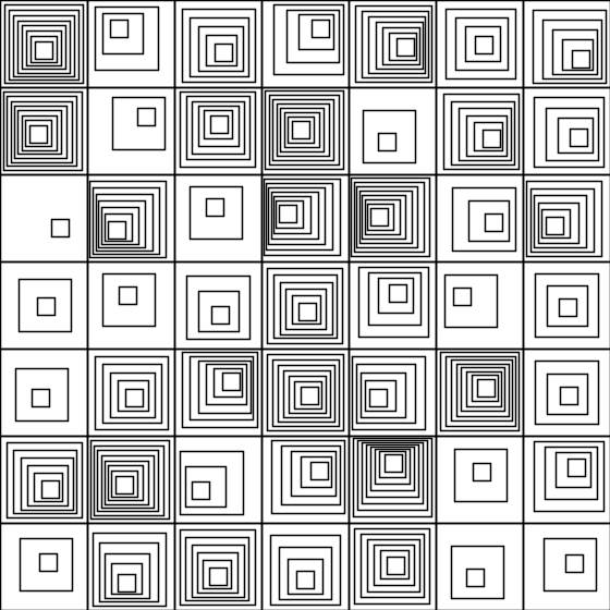
Random Squares
I recreated “Random Squares” by Bill Kolomyjec. You can see a picture of my creation below. The hardest part of this for me was getting it so there was only one cell that displayed a single square. I try to avoid while loops at all cost, and I had to mess around with while loops to get it working. Getting the squares to embed in each other was a little tricky as well. You can find my code here. Pardon the terrible variable names.
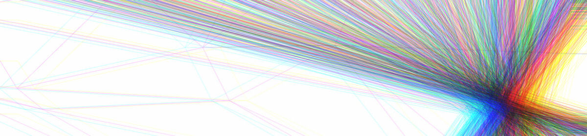
Lemme FFT that for ya
Here’s my self portrait:
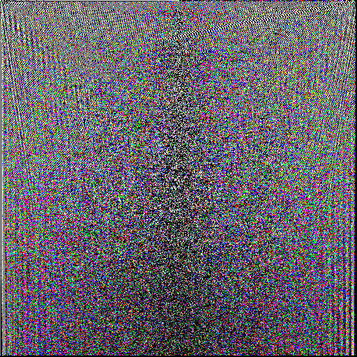
This actually contains the same information as the following image: